Blog entry 4: Design of Experiment (DOE)
- Ngo Van Anh
- Jan 22, 2023
- 7 min read

Welcome back, after the holiday, now it's time we get back to our adventure of making our chemical product.
This time, we will go on to obtain another skill to make our project come true. If all the last blogs involves learning some designing or fabrication skills to make the prototype, now we must learn how to test the prototype and identify how we can manipulate different factors for optimal results.
LEARNING REFLECTION:
The best way to learn is through practice, so that what this practical is about. We will be given a pre-designed set up, with 3 varying factors which can affect the results, and our task is to determine how much does each individual factor affect said results.
Our set up is a catapult, and we need to measure the distance travelled by the projectile in when we change certain factors to find out which combination of factors will give the furthest distance travelled.
The 3 factors are:
- Projectile weight (Heavy vs Light)
- Arm length (Long vs Short arm to launch the projectile)
- Stop angle (Large vs Small launch angle)
The specific details of each factor is provided to us on BrightSpace, we do not determine them ourselves.

After manually measuring the projectile weight, arm length, and stop angle, this is the data we obtained:
Projectile weight: 2g vs 0.86g
Arm length: 33cm vs 28cm
Stop Angle: 90° vs 55°
With 2 possible values for each factor, and 3 different factors, there are a total of 8 unique combinations, hence, 8 different runs to collect data. And to ensure the result we get is representative, we conduct each run 8 times and take the average distance travelled for the final result. We were split into 2 groups, me and Jeremy doing the Full Factorial method, where we collect 64 data points for the full set of data, and Jeevan and Yan Zhen doing the Fractional Factorial method, they will only collect data on 4 runs, meaning 32 data points, so already they are doing less work than us.

Our catapult set up

The projectiles are 3D printer, with the brown one being 0% infill and red is 100% infill

The different arms, which are also 3D printed

The complete setup, the tray contains sand the catch the projectile, and the distance travelled in measured by measuring from the projectile to the mark on the sand using a measuring tape.
After conducting 64 runs, this is the result me and Jeremy got
Full Factorial runs results:


Below is Jeevan and Yan Zhen's results, from the Fractional Factorial method:


Notice how in the runs they did conducted, their results is still different from our results of the same run, with their run 2 and 3 gives consistently and considerably lower results, with their run 2 average being 20cm lesser than our average. while run 5 and 8 only give slightly higher results.
While the discrepancy in run 5 and 8 is minimal and can be just random chance, the differences on run 2 and 3 is too great to just be random. We suspect it has something to do with the catapult.
Coincidentally, while trying to adjust the stop angle of the catapults, I accidentally take out the plastic elastic bands used to turn the axis of the rotating part where the arm is connected to. That is when we noticed that the elastic on mine and Jeremy's catapult is alot more tight and Yan Zhen and Jeevan's elastic band is more loose. This leads to my catapult being rotated at a higher speed and hence, launch the projectile at a higher speed, resulting in a further distance travelled.
We realized there is more than 3 factors affecting the distance the projectile can travel. However, it was explained to us during the lesson that ideally, we should only have 3 factors or less, so the number of experiment we need to run is not too many to be unrealistic. So in this experiment, how firm or loose the elastic bands are also contributed to the distance travelled by the projectile, but it was not taken into consideration, which is a good thing for us since it will be difficult to measure how elastic the bands are, and to obtain 2 bands of different elasticity to test.
To determine how influential each factor is to the result, we plot and compare graphs of the average results obtained when the factor is of high value vs when the factor is of low value.
From the Full Factorial data, the graphs are plotted like below:

To know how much does each factor affect the result from the graph, we see the gradient of each line. A steeper gradient shows a bigger change in distance travelled when the factor change from low value to high value.
Hence, from the Full Factorial method, the significance of the factors are ranked as:
Most significant ---> Least significant
Stop Angle > Arm length > Projectile Weight
Similarly, a graph was also plotted for the Fractional Factorial method:

And the ranking from the graph is also the same as the Full Factorial method. The gradient of the line for factor A and C is a bit difficult to differentiate with eyes, because with Fractional Factorial method there is less data. However, we used the display equation function in excel to make sure there is a gradient difference.
Finally, for our group challenge, we were given the task to knock down 4 targets of various distance. Using the data we collected, we need to set up the catapult so that the projectile travelled the correct distance to knock down the target. Much planning and strategy is required as we were only given a limited number of trials. We only ended up knocking down 2 targets out of 4, but it still places us into the second place and hence, securing us 8 additional points for the assignment.
CASE STUDY
Objective: Determine the most influential factor that affects the rate of popcorn yield out of 3 possible factors.
The factors and their High/ Low levels are:
Factor | High (+) | Low (-) |
A (Diameter of the bowl, in cm) | 15 | 10 |
B (Microwave duration, in minutes) | 6 | 4 |
C (Microwave power setting, in %) | 100 | 75 |
Data collected:
Run order | A | B | C | Bullets (gram) |
1 | + | - | - | 3.33 |
2 | - | + | - | 2.33 |
3 | - | - | + | 0.74 |
4 | + | + | - | 1.33 |
5 | + | - | + | 0.95 |
6 | + | + | + | 0.32 |
7 | - | + | + | 0.33 |
8 | - | - | - | 3.12 |
Full Factorial Method
To get the graph for factor A, we need to obtain 2 values: the average for all runs with A of High (+) value, and the average for all runs with A of Low (-) value.
The first point with High A will be = (3.33 + 1.33 + 0.95 + 0.32) / 4 = 1.4825
The second point with Low A will be = (2.33 + 0.74 + 0.33 + 3.12) / 4 = 1.63
Similarly, the points to plot the graph for B and C in obtained.

Then, the graphs are plotted to compare the gradients

From the graph, we can see that the graph for Factor C (Microwave Power Setting) is the steepest, at a gradient of 1.9425, followed by graph of Factor B (Microwave Duration), and finally, the least steep is the graph for Factor A (Bowl Diameter).
Hence, we can conclude that Factor C is the most significant in affecting the amount of bullets formed, Factor B is the second most significant, and least significant is Factor A.
Ranking: Most significant ---> Least Significant
Power setting > Duration > Bowl diameter
Interactions between factors
Beside influencing the final results, factors can also influence each other. To determine whether 2 factors influence each other, we can plot the graphs corresponding to the values of one factor (Factor X) when another factor (Factor Z) is High (+) or Low (-).
If both graphs plotted have a significant gradient from Low (-) to High (+) points, there is a significant interaction between the 2 factors., changing 1 factor also result in a change in the affect the other factor has.
However, if only 1 graph has a steep gradient while the other graph is horizontal or near horizontal, there is no or little interaction between the 2 factors, as changes in 1 factor does not result in changes in the effects of the other factor.
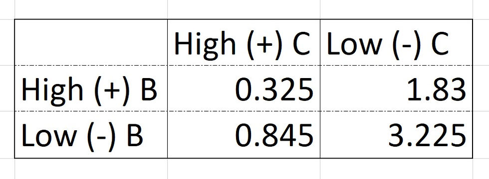
A x B Interaction

The values used to plot the graphs:

The graphs plotted:

From the graphs, we can see the gradients of the graphs are different, hence, there is a change in how A affect the amount of bullets depending on the value of B.
There is a significant interaction between factors A and B.
A x C Interaction


From the graph, both graphs has a steep gradient, hence there is significant interaction between factor A and C.
B x C Interaction


From the graphs, the graph for High C has a steep gradient, while the graph for Low C is a lot less steep. Hence there is some level of interaction, but not a lot of interaction between Factors B and C.
Fractional Factorial Method
For the Fractional Factorial method, run 2, 5. 6, and 8 were selected (highlighted in blue), as they have a good balance of values for all 3 factors. Each factor has 2 runs on Low (-), and 2 runs on High (+). Furthermore, Run 6 and 8 are good to cover as they are the 2 extremes combination, all Low values and all High values.

From there, the steps are the same as the Full Factorial Method:


From the graph, we can see that the graph for Factor A (Bowl Diameter) is the steepest, at a gradient of 2.09, followed by graph of Factor C (Power Setting), and finally, the least steep is the graph for Factor B(Duration).
Hence, we can conclude that Factor A is the most significant in affecting the amount of bullets formed, Factor C is the second most significant, and least significant is Factor B.
Ranking: Most significant ---> Least Significant
Bowl diameter > Power setting > Duration
CONCLUSION: As we can see, the Full Factorial method and the Fractional Factorial method sometimes can give different answers as to what factor has the most influence over the final result. This is due to in Fractional Factorial method, we do not try every combination of factors possible, but only pick some, which could lead to a bias in the result. This compromise is something we need to keep in mind when doing Fractional Factorial, even though it is easier and less time and resources consuming to collect less data points, it might not be as representative as the Full factorial method.


Comments